7 · The number Draft
Coordinated omission
On this page
Coordinated omission
The worst failure has a name, and it comes from how the harness offers messages to the program. A closed-loop harness sends a message, waits until the program has finished with it, records the time, and only then sends the next, so each start depends on the previous end. An open-loop harness sends each message at a time fixed in advance, whether the program is ready or not. Most first harnesses are closed loops, because for m in msgs { let s = now(); handle(m); record(now() - s) } is the obvious way to write one.
In a closed loop the sending is coordinated with the program’s progress. When the program stalls, the harness waits with it, so the messages that would have arrived during the stall, and waited, are never sent, and their latencies are never recorded: they are omitted, in coordination with the stall. Gil Tene named this coordinated omission. Here it is with a message every 10 µs, 0.3 µs to serve each, and one stall of 10 ms:
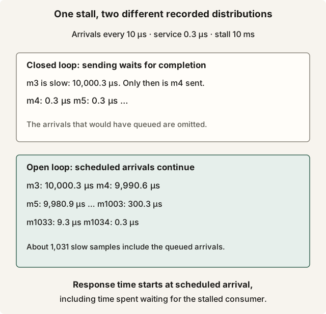
One stall, two different recorded distributions. Select the diagram to open it at full size.
In the closed loop, m3 is recorded once, at 10,000.3 µs, and m4, sent when m3 is done, is recorded as 0.3. Whether the harness then skips the slots it missed or sends the late messages in a rush, each is timed from when it was sent, after the stall, and none of them waited. In the open loop, m4 arrived at 40 µs and finished at 10,030.6, so it is recorded as 9,990.6 µs. The backlog drains at 0.3 µs a message while new ones keep arriving every 10 µs, so it clears at m1034, and 1,031 messages land evenly between 10 ms and nothing.
The two loops measure different things. m4’s service time, from the moment the loop started on it to the moment it finished, is 0.3 µs. Its response time, from its arrival to the moment it finished, is 9,990.6 µs, of which 9,990.3 is waiting. A closed loop measures service time and reports it as latency. Over the second that holds the stall, 100,000 messages, the closed loop’s histogram reads p99 0.3 µs, p99.9 0.3 µs and max 10 ms: one bad sample, the kind that gets called noise. The open loop’s reads p99 0.3 ms, p99.9 9 ms and max 10 ms. Same program, same stall, and the two p99.9s differ by a factor of 30,000. Both are worth reporting: service time says how fast the loop is once it runs, which is what to optimise, and response time what the market experienced, which is the product.
The fix is the open loop: messages arrive on their own schedule, and latency is measured from the scheduled arrival, not from when the loop picked the message up. The schedule must resemble production, and only the market’s own does, which makes a replay file with recorded arrival times the only honest input. A constant synthetic rate is an open loop without bursts, and it understates every percentile the bursts set; “as fast as possible” has no schedule to be late against. The capstone’s paced mode computes t0 as start + ticks(t_arrival_ns) rather than reading it, so a feed thread held back by a full ring cannot hide its own lateness. --stall-every 1000 puts the same 10 ms stall into the real loop once a second, so that think, the loop’s service time, and total, the message’s response time, can be read side by side; the worked example below gives the prediction.
A closed-loop harness that cannot be changed can be patched: the hdrhistogram crate’s record_correct(value, interval) records a value and, when it exceeds the expected interval between messages, the samples the stall would have produced, the value minus one interval, minus two, down to the interval. It assumes evenly spaced arrivals, so it is an estimate; the open loop is the measurement.