7 · The number Draft
Latency endpoints and distributions
On this page
7.1 What a latency is to a program
A latency is the time between two moments in the life of one event, and a program that measures one has to choose both moments before it reads any clock. Everything else in this chapter, the counter, the histogram, the ways a number lies, comes after that choice and cannot repair a bad one.
Two points in time
An event is one thing the program handles from start to finish: a market-data message, a web request, a frame of a game, a query. Its latency is the time from a chosen start point to a chosen end point, for that one event. Neither point is given by nature. A depth update for BTC-USDT-PERP passes many moments a program could call its start: the last bit of its frame arriving at the network card; the kernel copying its bytes into the program’s buffer; recv returning; the decoder finishing; the book changing; the strategy deciding; the order’s bytes handed to the kernel; the order’s frame leaving the card. The trade’s name for the whole of it, from the frame in to the order’s frame out, is tick-to-trade. Each earlier start includes more of the path, and each later end includes more of the response.
A program can stamp only the moments it can see. It cannot read a clock at the instant the card received the frame, because nothing of the program runs then; it learns of the frame microseconds later, when the kernel hands it over. Cards that stamp frames themselves exist, and they belong with the things this chapter leaves out. What a program can do is take its start at the earliest point it owns and say exactly which point that is.
The capstone takes application-arrival-to-decision: from the moment a message’s bytes are handed to the program, which it calls t0, to the moment the strategy’s decision about it exists, t3, whether that decision is an order or a choice to send nothing. The kernel’s receive path is before t0 and the send path after t3, so neither is in the number. Between t0 and t3 the capstone marks the boundaries of the stages too, decode done and popped on the strategy’s core, so that a slow total can be split into the stage that was slow.
A latency quoted without its two points is not yet a number. “Apply takes 3 ns” and “the update took 300 ns” can both be true of the same update: the first runs from the call to apply to its return, the second from the bytes to the decision, with a decode, a ring hop, a quote and two clock reads around the apply. Two variants of a program can be compared only between the same two points.
One number per event
A run of a million events produces a million latencies, one sample each, not one latency. What the run measured is a distribution: for each value, how many samples took it. A distribution is most easily seen as counts per range of values, and a million updates through a strategy thread on a pinned core look like this:
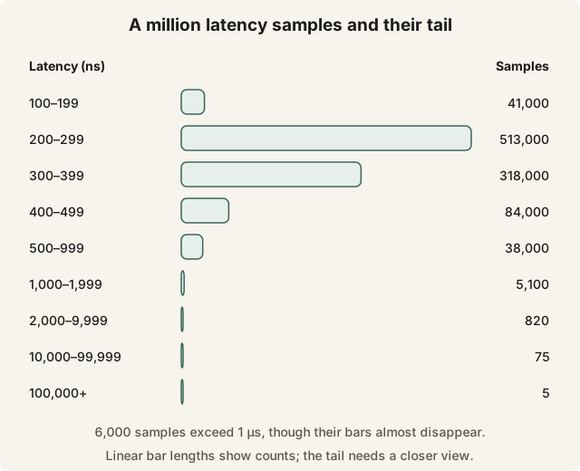
A million latency samples and their tail. Select the diagram to open it at full size.
The shape is typical of latencies anywhere. There is a floor, here a little over 100 ns, set by the work itself: the instructions the path executes and the lines it loads, which nothing makes faster. Most samples sit just above the floor, because most events find their lines in cache and nobody in the way. Above the peak there is a long, thin tail, because everything that can happen to an event adds time and nothing subtracts it: a cache miss adds 80–100 ns, a line still owned by another core 50–100 ns, an interrupt a few microseconds, a preemption milliseconds. So a latency distribution is bounded on the left, crowded near the floor, and stretched to the right over four or five powers of ten. It is not a bell curve, and the vocabulary of bells, a mean and a standard deviation, describes it badly.
Drawn to the scale of its peak, the tail is invisible. The 6,000 samples above 1 µs would need a third of one # between them, yet they are the samples the rest of this chapter is mostly about.